Phase 1 · complete
Replication with corrections: the neural network
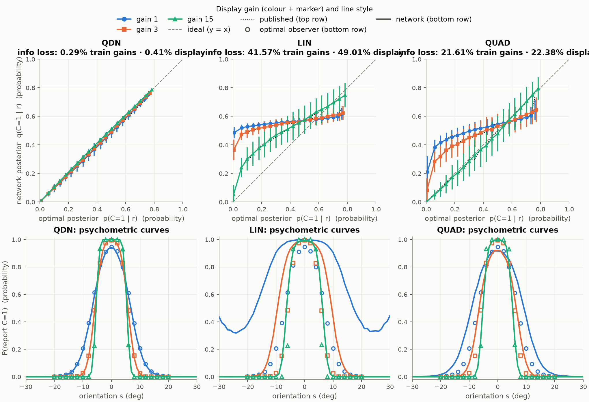
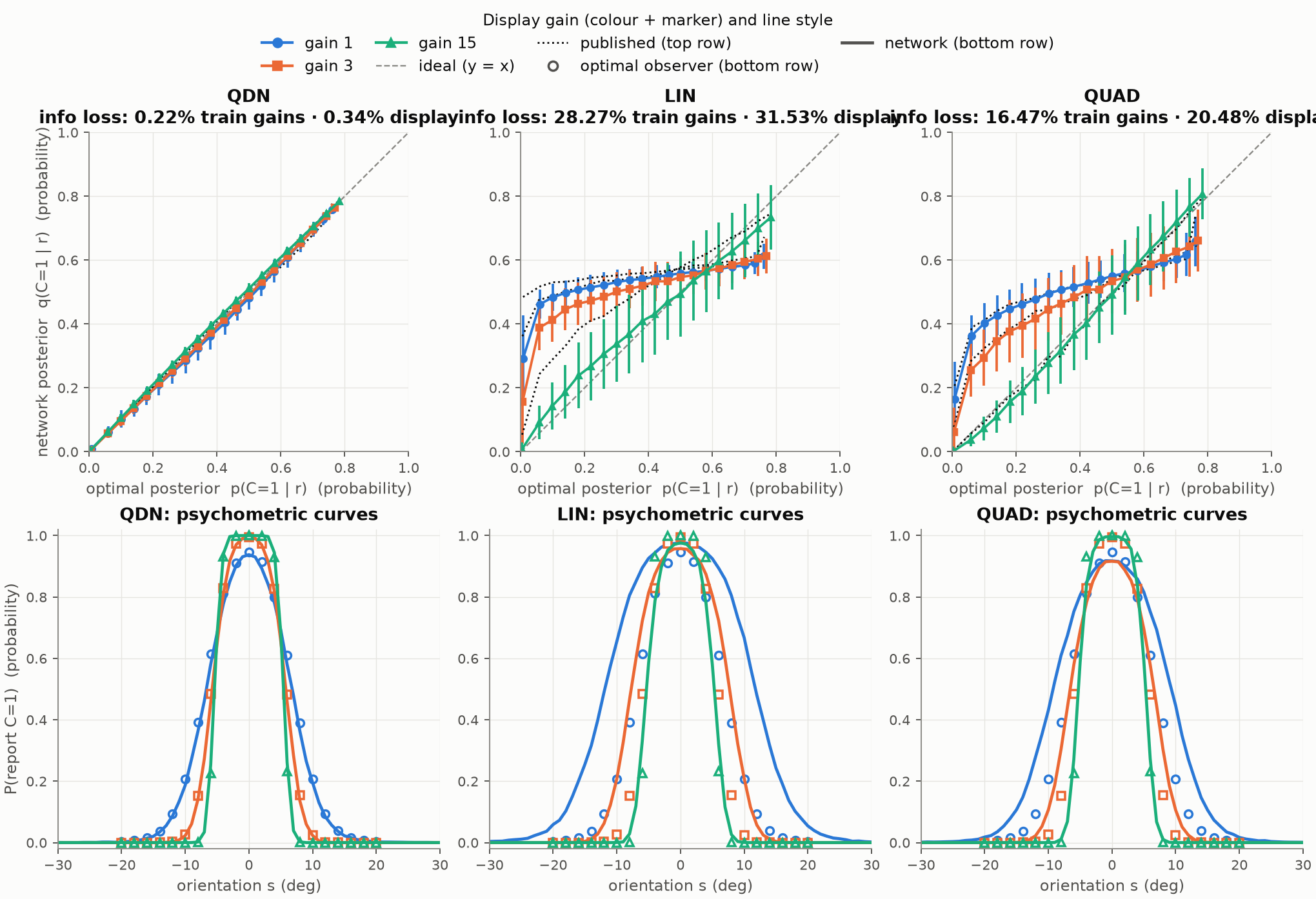
All three published information losses reproduce. With a working optimiser QDN stays near-optimal, but LIN and QUAD turn out to have been undertrained, the size of the gap depends on the range of gains, and divisive normalization does not "emerge automatically" through learning.
Set-up
A population of 41 Poisson neurons with Gaussian orientation tuning (, preferred orientations to ) encodes the stimulus. The gain, which plays the role of contrast, takes six values from 1 to 32. The optimal decision variable written in terms of the population activity is
with and . Its second term is a quadratic function of activity divided by a quadratic function of activity: a divisive normalization. Three networks read out from the population: LIN (linear in ), QUAD (all pairwise products ), and QDN (quadratic numerator over a quadratic denominator). Performance is the information loss: how much worse the network's posterior over the category is than the optimal posterior, as a percentage.
Published vs replicated vs corrected
"Faithful" re-implements the archived training code, including its update rule and iteration counts. "Corrected" removes the confirmed bugs and trains to convergence with Adam on soft targets. All values are tested on 105 trials at the six training gains.
Information loss by network
Percent, lower is better. Values at the bar ends; hover for details.
The LIN problem is convex, so its optimum can be computed exactly: ,
which is where the corrected training ends. The QUAD optimum could not be computed exactly (the streaming Newton solver had not converged
at its iteration cap); the converged training value suggests the asymptote is at or below about 16%. The archived authors' own
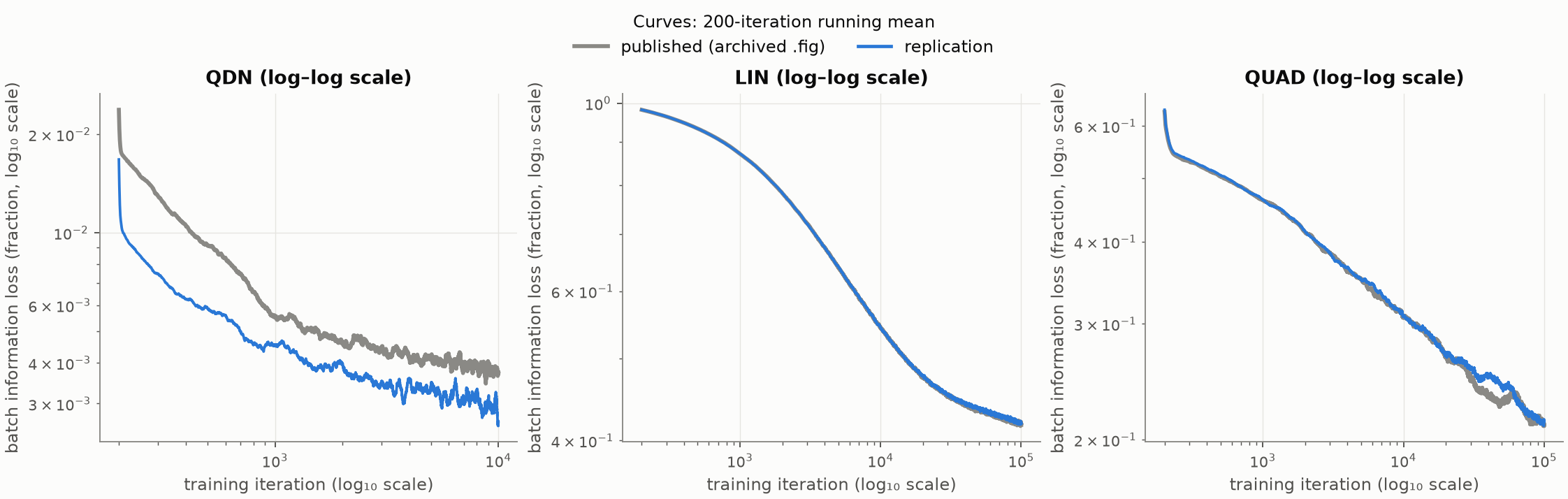
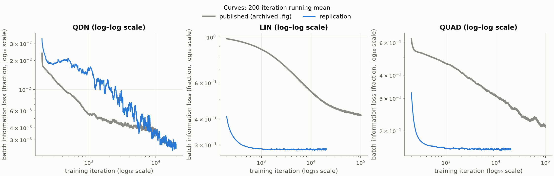
curve fit (in the archived figure file FigN_s1) placed LIN and QUAD 91% and 87% of the way to their asymptotes, which contradicts the SI's
"close to the asymptotic ones".
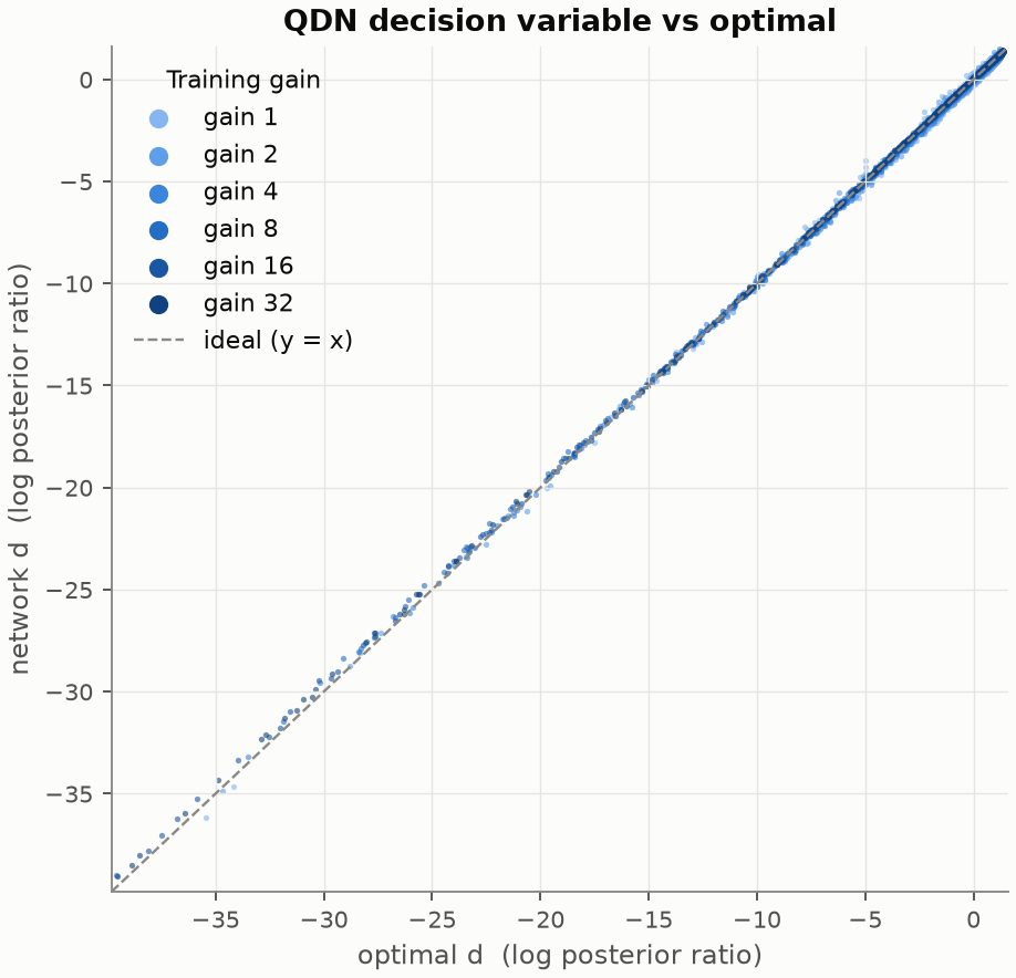
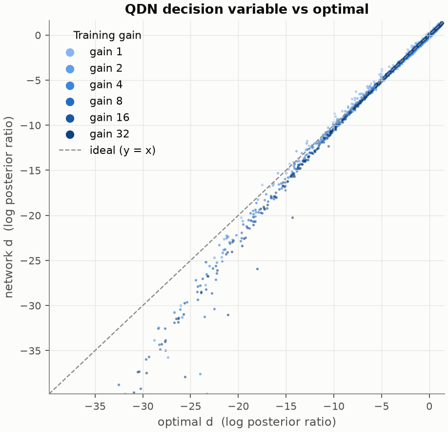
Conclusion: "QDN is near-optimal" holds (0.22% corrected). "LIN and QUAD are not" holds qualitatively but was overstated: the true values at six gains are about 28.5% and 16%, still 60–130 times the QDN loss.
Reconstructing the missing QDN script
The archive contains the paper's LIN and QUAD scripts but not its QDN script (six gains, initialisation "according to Eq. 6", 104 iterations). The SI has no numbered Eq. 6. The archived figure file for Fig 5 is titled "QDN2, Taylor IC: 0.38631%", and a second figure file holds its full learning curve, which starts at 60.0% loss.
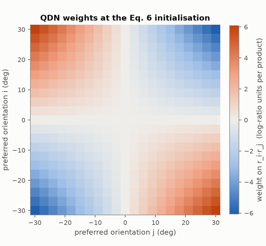
The agent built the network the SI describes, , and read "Eq. 6" as the optimal decision variable written in neural terms (the SI text says "substituting … into Eq. 3 gives us Eq. 6"). Setting , and to the exact second term of makes the network start at information loss, against 60.0% in the archived curve. That match is strong evidence for this reading. The learning rate could not be recovered (the archived rate does not move the network at all), so it was chosen to match the archived curve's first iterations. The faithful QDN number is therefore partly tuned, not an independent reproduction.
The gap depends on the range of gains
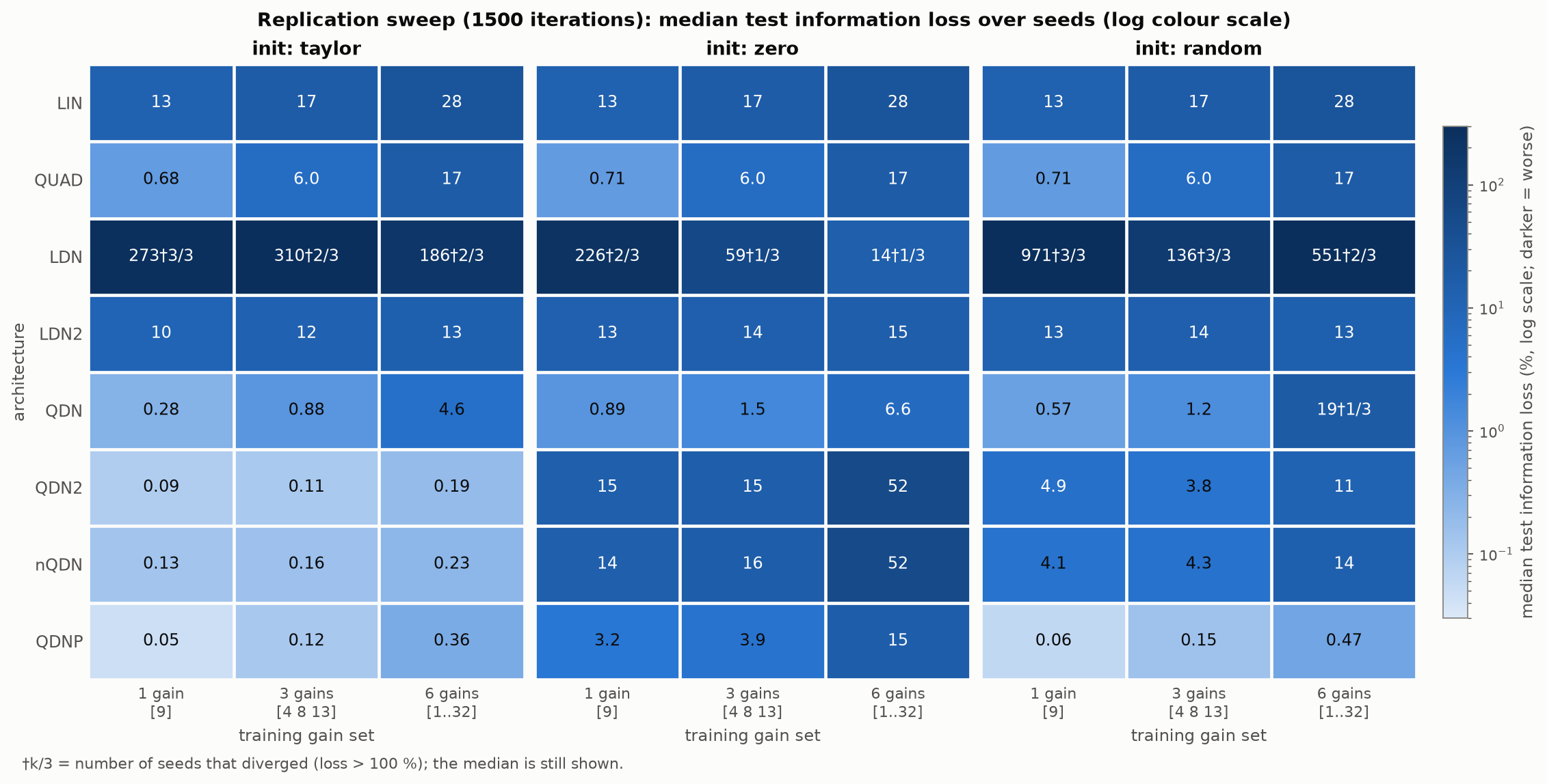
The paper's contrast (QUAD 21% vs QDN 0.39%) belongs to the six-gain setting. A sweep over gain sets (1500 Adam iterations, 3 seeds, median) shows how quickly QUAD's disadvantage shrinks when fewer gains have to be handled by one readout.
Information loss vs number of training gains (log y)
Median over 3 seeds; information loss on a log scale. Gain sets: [9], [4 8 13], [1 2 4 8 16 32]. Networks start from the paper's initialisations.
Does divisive normalization "emerge automatically"?
Not as a learning result. The phrase is accurate for the mathematics and not for learning:
- The basis is chosen by hand, and its second term is the optimal written out.
- The paper's QDN starts at the exact optimal numerator and denominator of that term. The training from 60% to 0.3% loss is the network learning the log term, not the normalization.
- Started without that knowledge, the normalization networks do learn an activity-dependent denominator, which grows with total spike count, and they beat QUAD. But they stay 5–30 times short of the analytic start within the paper's 104-iteration budget, and were still improving. Whether longer training closes the gap is open (one seed per initialisation).
Same architecture, different starting points (104 iterations)
Test information loss, %. "Slope" compares the learned and optimal denominators (log–log; 1 = matches the optimum). QUAD (converged) for reference.
QDNP "random" draws each denominator element uniformly between 0 and twice its optimal value, so it is centred on the optimum and is not an uninformative start. QDN2 "jittered zero" perturbs the archived zero initialisation slightly and is uninformative.
The "General network" and its lesions (Full, L1, L2, L3, T3)
The archive holds figures labelled Full, L1, L2, L3 and T3 with no surviving script. The agent identified them from the archived figure files, the
2010–2012 drafts and slides (reports/nn_variants_full_L_T.md). They are not Taylor orders but a lesion study of a three-term
"General network" that the drafts describe:
- Full uses all three terms; L1, L2, L3 remove one term each and retrain.
- T3 only is the divisive-normalization term alone, and it is the published QDN (the SI's basis is T3 renamed).
- "Taylor" and "Random" in the archived panel titles are initial conditions. The Taylor start expands the log term of the optimal d to first order in 1/(a·r) (giving T1 and T2) and sets T3 to the exact divisive-normalization term of d.
Without T3 nothing useful can be learned: L3 sees only total spike count, which carries no category information, and loses about 100% (the best possible function of total count loses 100.2%). T3 alone is near-optimal. The two extra terms help a little, by approximating the log term that T3 lacks.
General-network lesion study: archived vs reproduced (log x)
Information loss (%, log scale). Archived: bars in the archived figure file (104 iterations). Reproduced: 2,000 Adam iterations, tested at the six training gains. L3 is left out of the chart: it diverged in our runs (archived: 100%); see the table.
Table view
The lesion pattern reproduces: L3 is worthless, L2 ≈ Full, T3 alone is near-optimal, and L1 is worst of the rest. The archived Full network's 0.008% is not reproduced at 2,000 iterations (ours: ). Three different T3 numbers exist in the archive (0.29%, the 1.14% of a 2012 draft, and the published 0.39%), and it does not say which runs or test sets produced them.
Network code audit (N1–N8)
From the network-replication agent and its own independent reviewer. File and line references are in reports/nn_replication.md §6.
| # | Severity | Finding | Status | Impact |
|---|
Speed
The archived MATLAB logged its own speed: 2.07 s per training iteration of 7,000 trials, with the basis built in a per-trial loop. A 2.56-million-iteration run took about 61 days of compute. The JAX re-implementation takes ms per 10,000-trial iteration on one core, about 65–110 times faster per trial across network types. The whole faithful replication (2.1×10⁹ simulated trials) ran in 41 minutes on 3 single-threaded processes.
Figures
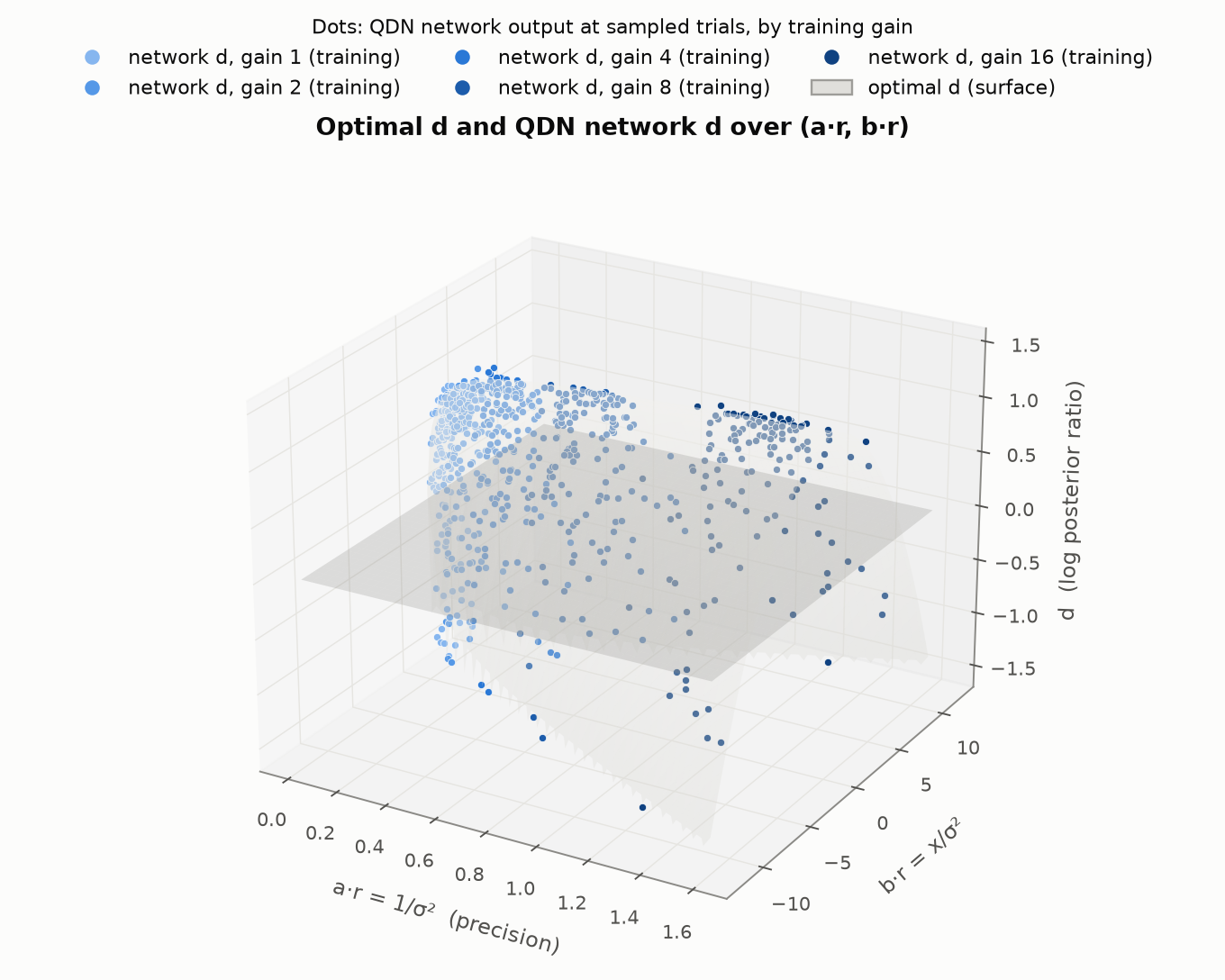
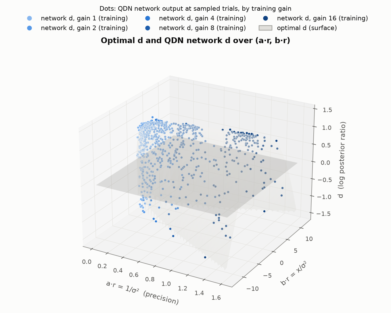
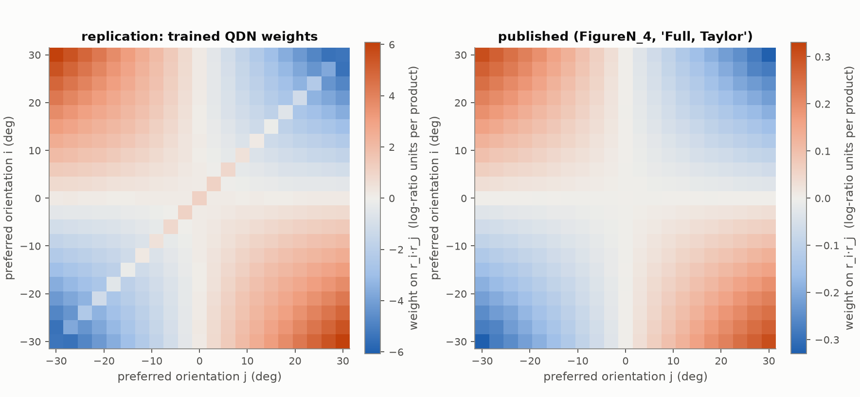
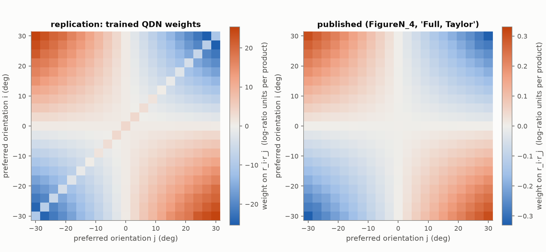
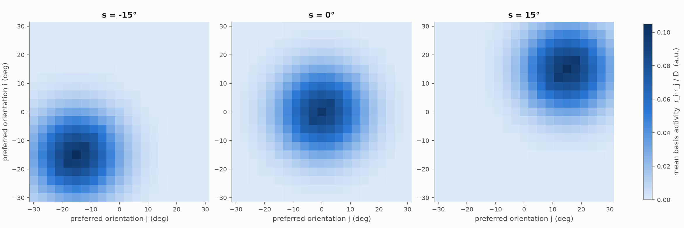
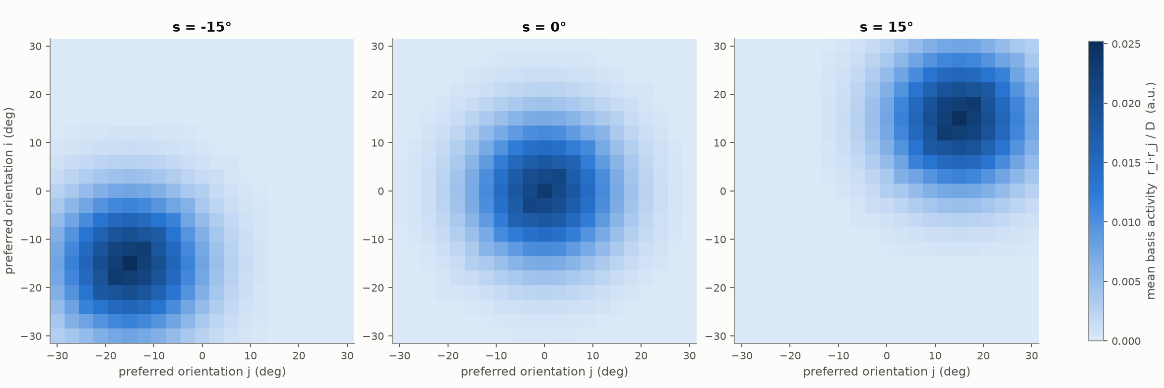
All network figures were redrawn after the networks were retrained (the retrained numbers reproduce the Phase-1 values). Faithful = the archived training code re-implemented; corrected = bugs removed, trained to convergence.
Phase-3 network figures (generic networks, learning signals, circuits, contrast generalisation) are on the Extensions page.