Phases 2 and 3 · complete
Extensions
The 2013 analysis left open why subjects split between the optimal rule and heuristics. Phase 2 tests near-Bayesian and noise explanations, adds trial history, and checks whether the models can be told apart at all. Phase 3 asks whether the network results hold up for generic, biologically plausible networks. Each result is tied back to a claim in the paper.
Phase 2 in one paragraph. Adding noise to the optimal observer does not explain the data: the best noise model
loses to the best paper model by (Monkey L) and
(Monkey A) in . A Bayesian observer that over-weights its own
uncertainty ( ≈ ) matches the best heuristic in Monkey A only; in humans it is clearly better for no one (AJ's narrow tie is uninformative), and where recovery
shows it could be identified (RG, JO) the data reject it. A mis-learned-category model is favoured for one subject (TS) under one prior box only. Trial history is real in 7 of 14 subjects but changes no model comparison. Full write-up:
reports/phase2_models.md.
History effects and the trial-order discovery done
The paper's models treat trials as independent. Whether real observers carry information from one trial to the next can only be tested if the stored trial order is the order in which trials were presented.
The agent's first claim was wrong
The agent first logged "trial order verified": subject MR's orientation sequence repeats exactly every 648 trials, one session, which looked like
presentation order. Checking against the raw 2009 session files showed otherwise. Each block was presented section by section (3 sections × 72 trials),
but the loading code (readdata.m) flattened each block's matrix column-major, interleaving the sections. The 648-trial repeat holds under either
order, so it proved nothing. The agent corrected the log, reconstructed the true order exactly (scripts/verify_trial_order.py), and a forensic
subagent showed the control experiment is interleaved the same way (3 × 96 per block), while the monkey data are chronological.
This has no effect on the paper's analyses, which assume independent trials. It matters for sequential effects: in the stored order every human subject looked history-free.
What the true order shows
A logistic regression of each choice on the fitted model's decision variable plus the previous response, split by whether the previous trial was correct. The model coefficient stays at about 1 for every subject (the fitted models are well calibrated). In true order, of humans show strong sequential dependence (likelihood-ratio test, p < 0.001): four repeat their previous response and two alternate. Monkey L perseverates, more strongly after errors; Monkey A shows nothing.
Effect of the previous response on the current choice
Logistic-regression coefficient, ±1.96 SE. Positive = tends to repeat the previous response; negative = tends to alternate. Bold names: p < 0.001.
Table view
Does modelling history change the model comparison? No.
Each paper model was refitted with the same two history weights inside its likelihood ("+H" models). History improves every model by at least 5 nats () in exactly the seven subjects the regression flagged. The winner changes by AIC only for three subjects whose base models were already tied within 1 nat (MR, RB, WJM), and by Laplace evidence for none. Monkey L's Lin-σ win survives: Lin-σ+H beats Quad-σ+H by . Nested evidence is not used here: every Lin-σ+H and Quad-σ+H nested run hit its call budget and is treated as missing.
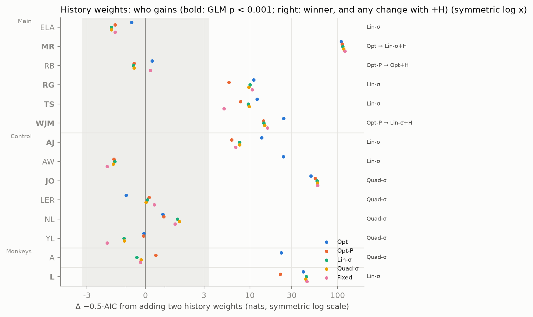
Table view
Near-Bayesian and noise models done
Every model keeps the paper's measurement noise and lapse rate, contains Opt as a special case, and turns one explanation of the departure from Opt into a parameter:
- ImpSigma: the Bayes rule applied to a distorted uncertainty estimate . is Opt, a fixed boundary, over-reaction.
- Mismatch: the Bayes rule with wrong beliefs about the category widths, and .
- Noise on Opt: Gaussian decision noise on the log posterior ratio (DecNoise), a softmax readout (Sampling; is posterior probability matching), a trial-to-trial noisy uncertainty estimate (NoisySig), and fluctuating precision that the observer knows (VarPrec).
Fits: maximum likelihood (300 random starts); scores: , Laplace evidence (only where the optimum is interior with a positive-definite Hessian) and nested-sampling evidence (only for runs that converged within the call budget).
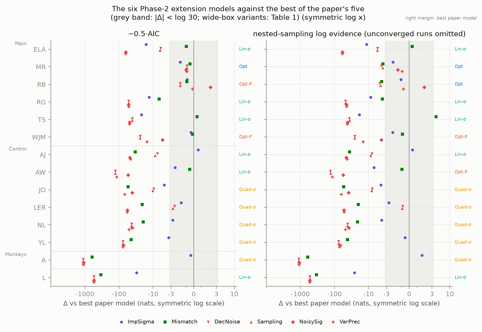
Table view (Δ vs the best paper model)
Noise does not explain it. No noise model beats the best paper model by AIC in any subject except NoisySig for RB (). In both monkeys decision noise collapses to zero, and the best noise model loses by (Monkey L) and (Monkey A). Some humans do have decision noise, but it does not fix the shape of their boundary. The departure from Opt is a systematic distortion of the decision rule, not noise around it.
Misjudging one's own uncertainty (ImpSigma)
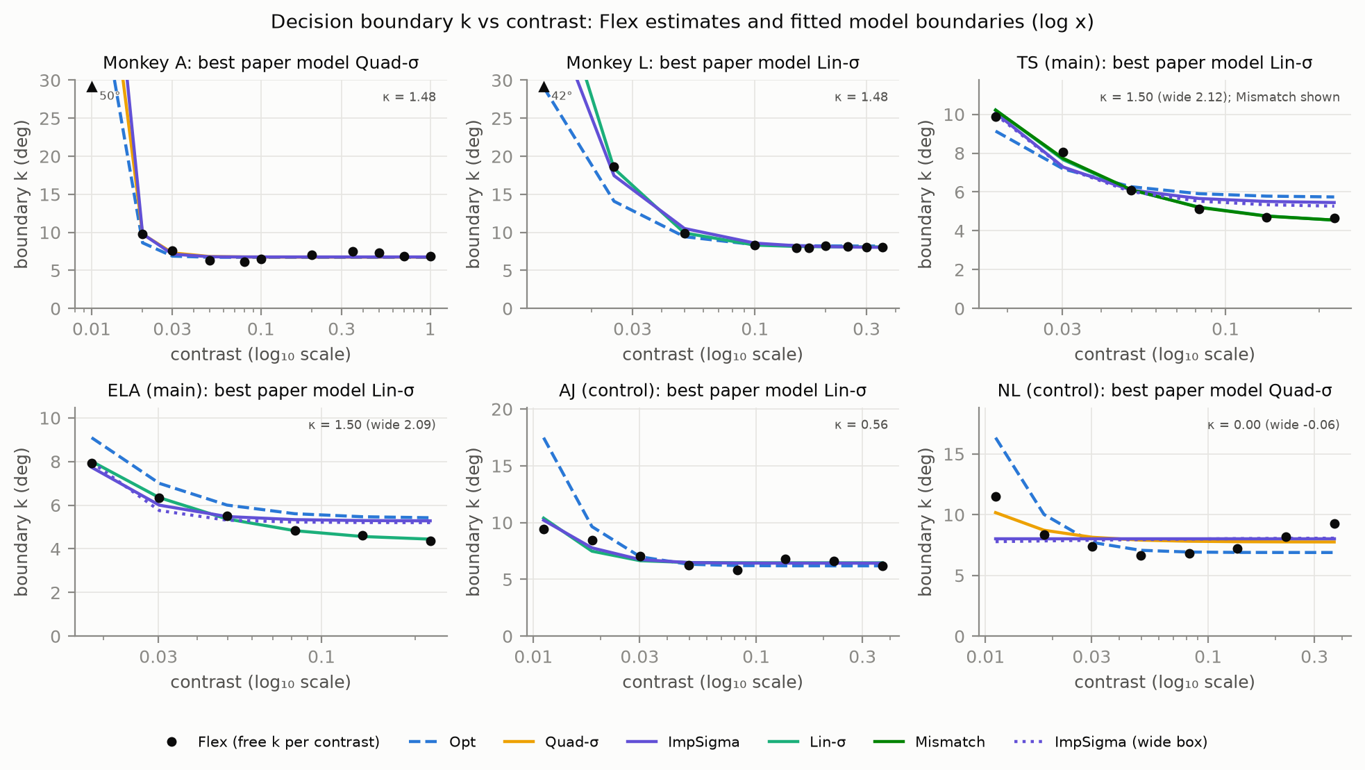
ImpSigma matches the best heuristic only in Monkey A ( against Quad-σ by AIC, by nested evidence, below ). Monkey A was not in the recovery study, so this tie cannot be checked against simulated data. It also ties for control subject AJ ( AIC, nested), but that tie is uninformative: ImpSigma simulated at AJ's own fit is called Lin-σ in 4 of 4 datasets, and ImpSigma wins 3 of the 20 datasets simulated at AJ's parameters from the other models. Monkey L prefers Lin-σ (ImpSigma by AIC, nested).
Both monkeys over-react to uncertainty: = ± (Monkey A) and ± (Monkey L) in the wide box (untruncated posterior SD), the same value as in the original box. For Monkey L this comes from a model 26–31 nats worse than Lin-σ. A check that uses no boundary model agrees: both monkeys' free per-contrast (Flex) boundaries lie above the optimal boundary at the lowest contrasts and close to it at high contrast.
Human values are fits, not traits. ImpSigma is clearly better for no human, so each belongs to a fit with the Δ against the subject's best model given in brackets: NL (−2.8, a fixed boundary), JO (−4.7), AJ (+0.6, uninformative), LER, MR, RB, WJM and AW near 1 (−0.4 to −2.5), YL 1.45 (−3.5), RG 1.55 (−12.9), and in the wide box ELA (−13.9) and TS (−16.1). The Flex check supports over-reaction for RG and YL, only weakly for TS, and not for ELA (its Flex boundary is below the optimal one at every contrast); it supports under-reaction for JO, AJ, LER and NL.
: how strongly the boundary tracks uncertainty
Maximum-likelihood ± nested posterior SD, original box (0–1.5) and wide box (−1–4). 0 = ignores uncertainty (Fixed), 1 = optimal (Opt).
Caveat: in humans, whether ImpSigma can be identified depends on the subject. In model recovery (below) it is recovered 4 of 4 times at RG's and JO's fits, where the real data reject it (by 13.0 and 4.7 nats): identifiable, and rejected. It is unrecoverable where it is nearly Opt (MR, RB) or nearly Fixed (NL: called Fixed 4 of 4 times), and at the ELA, TS, AJ, AW, WJM and LER fits. Pooled, ImpSigma datasets are recovered (main) and (control) of the time; with Monkey L's trial count, .
Mis-learned categories (Mismatch)
The monkeys reject it ( and by AIC): to make the boundary grow at low contrast it needs an absurdly wide second category, and its belief runs to the edge of the box. Four control subjects put the width ratio at its lower edge (1.01). For subject TS, Mismatch is favoured by evidence under the original box only: there it beats every paper model by (nested) and (Laplace), above , with believed widths of ° and ° instead of 3° and 12°. Under the wider box the same fit scores (nested) and (Laplace), below , and by AIC it is a tie (). Lin-σ and Mismatch reach nearly the same likelihood, so the gap is prior volume. Mismatch was not in the recovery study.
Wider parameter boxes
The first fits put at its upper edge (1.5) for three humans and the Mismatch ratio at 20 in six fits, so both models were refitted with wider boxes (, ; ). Because the box is the prior of the evidence, both versions are kept. One conclusion changes: TS's Mismatch advantage drops below (above). moves only for ELA, TS and RG, which still lose to Lin-σ by 13–16 nats. Under nested evidence two winners change by small margins (RG to the wide Mismatch, ; AW by 0.2).
Winner among all 13 models, per score
Model recovery done
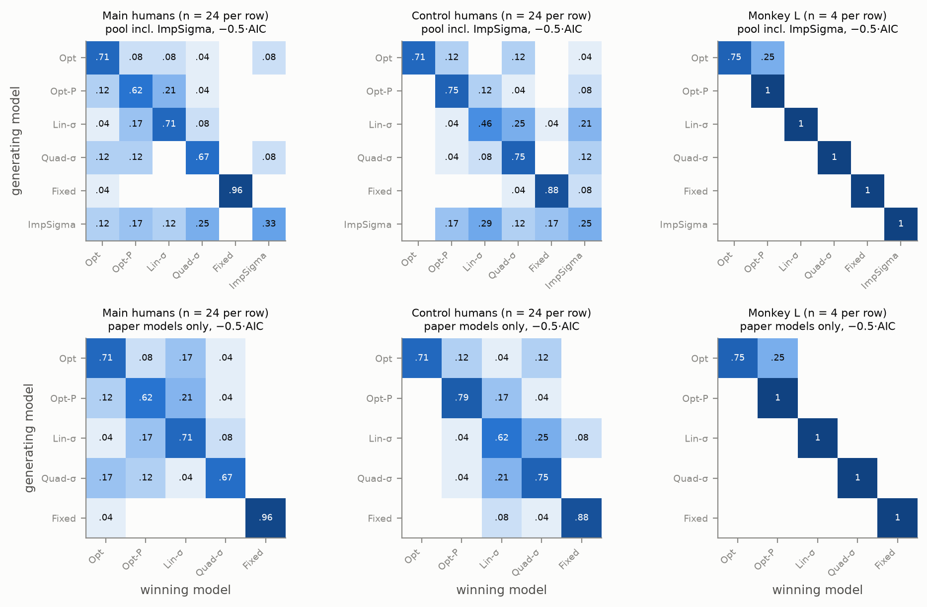
Synthetic datasets were generated from each model at each subject's own fitted parameters and on that subject's own stimuli (4 per subject and model), then every model was refitted. This tests whether the design and trial counts can tell the models apart.
ImpSigma recovery per subject
The paper's models are recovered reasonably in humans and well in Monkey L. Fixed is the easiest; Lin-σ in control humans is the hardest (, often called Quad-σ or ImpSigma; when ImpSigma is not a candidate). The refits use a reduced protocol (200 starts) and AIC/BIC, not evidence. ImpSigma also produces false positives: in control humans it wins 13 of the 120 datasets simulated from the other five models, against 6 of the 24 simulated from ImpSigma itself (main humans: 4 of 120 against 8 of 24).
Evidence methods
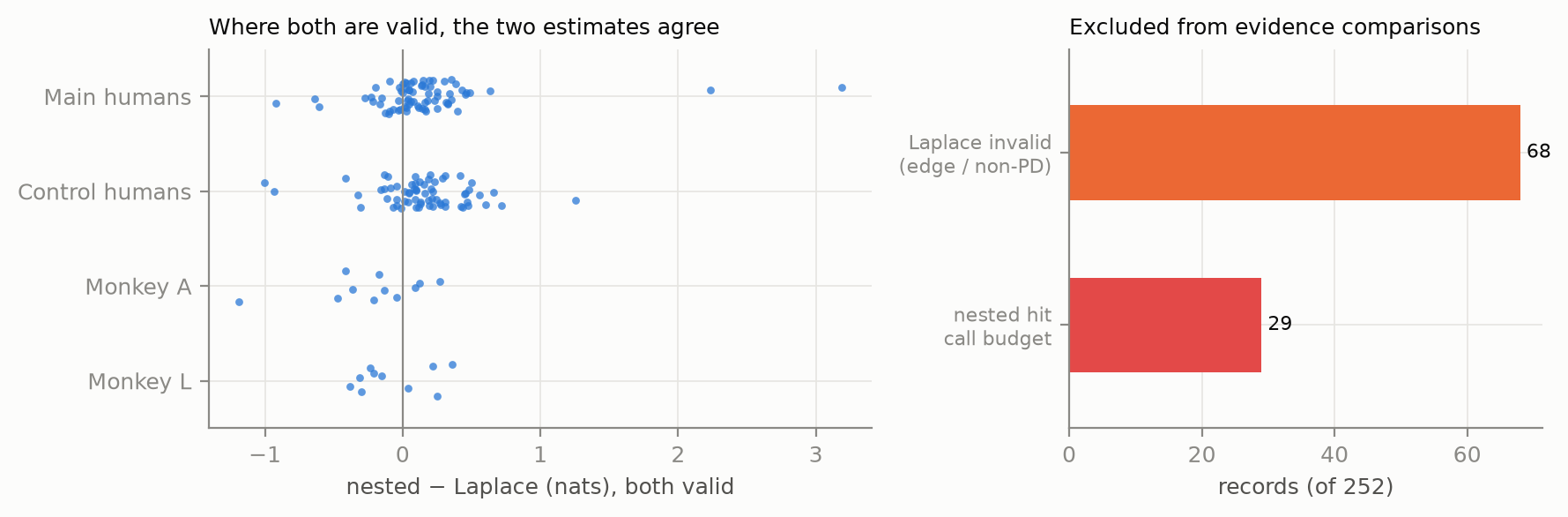
Across the Phase-2 fit records (paper, extension, wide-box and history models), nested sampling and Laplace agree to a median of nats where both are valid ( records; 95th percentile ). Laplace is invalid for records (optimum on a box edge or a non-positive-definite Hessian). nested runs hit the 3×10⁶-call budget; they are treated as missing, not as low evidence. The nested runs use orientation-binned data plus a correction evaluated at the best fit, which carries an error of at most a few tenths of a nat (largest correction: nats, Monkey L).
Neural-model extensions (Phase 3) done
Seven experiments on the paper's network claims, all on the paper's task and 41-neuron Poisson population (full report: reports/phase3_neural.md).
How it integrates with the paper. "QDN is near-optimal" holds but is not special: generic networks trained from random starts do better in range. "Divisive normalization emerges automatically" is not supported as a learning or circuit result. Networks that are near-optimal but limited in capacity, data or teaching signal look like Quad-σ or Lin-σ observers, and Fixed never wins, which supports the paper's "observers use uncertainty" conclusion while weakening its contrast between Bayesian and heuristic observers.
Contrast generalisation (E7): architecture or initialisation?
In E1 the paper's QDN extrapolated to gains it had not been trained on, while generic networks failed. But that QDN started at the analytic solution. E7 separates the two. The claim has to be tempered. The analytic numerator is unnecessary: a random readout over a uniform, non-negative normalisation pool at 0.1–10 times the analytic scale extrapolates like the analytic QDN, even when the pool is frozen. But that random pool equals the analytic pool in expectation, so the result is not independent of the initialisation. Genuinely non-uniform pools generalise much worse, especially to lower contrasts. What carries contrast generalisation is normalisation by approximately uniform total population activity, not the full analytic solution. A generic MLP fed ( is a learned constant, written in the Phase-3 report) generalises best of all. Orhan & Ma (2017) saw transfer because they trained at full contrast and tested only lower contrasts; our generic networks pass that test too but fail above the training gain.
Extrapolation to unseen gains (log x)
Information loss (%, log scale), mean of 3 seeds. "Up": trained on gains 1–4, tested at 8–64. "Down": trained on 8–32, tested at 0.5–4.