Phase 1 · complete

Replication with corrections: behaviour

Every published behavioural number was reproduced from the archived data and code. The audit found real bugs, and fixing them changes several numbers. It changes no model winner and no main conclusion, though three claims need qualifying.

Task and models
Faithful replication
Code audit
Corrected vs published
Boundaries
What changed
Figures

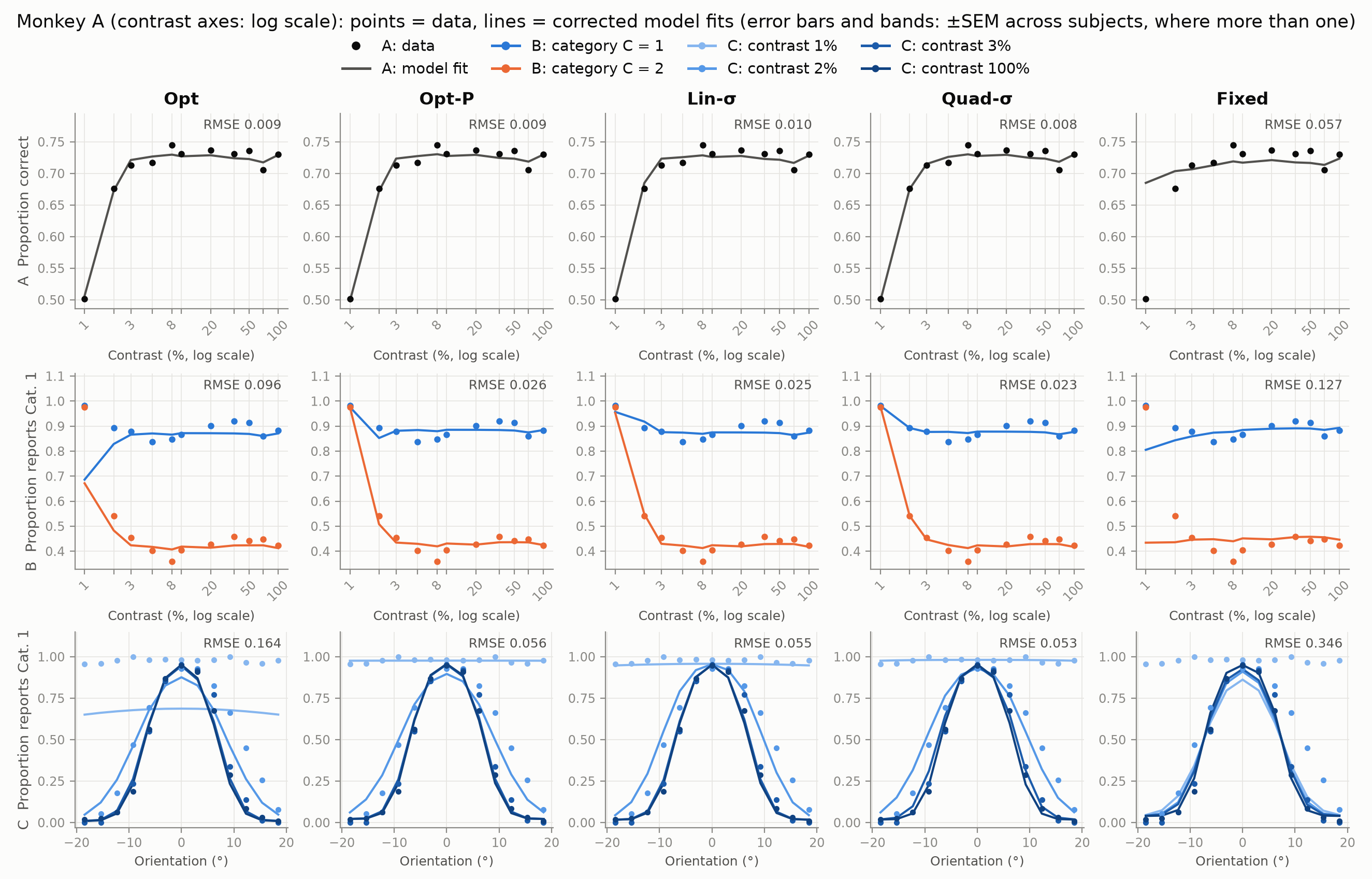
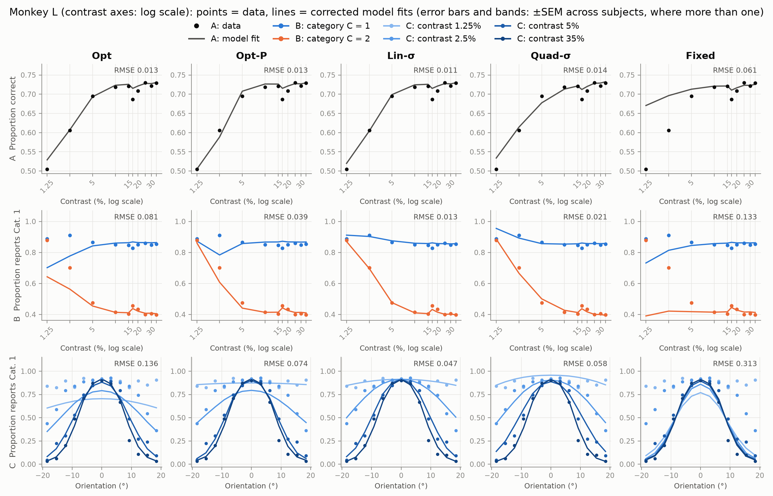
The task and the five models

On each trial a category $C$ is drawn (1 or 2, equally likely). Category 1 orientations are tightly clustered around horizontal ( $\sigma_1 = 3^\circ$ ), category 2 orientations are spread wide ( $\sigma_2 = 12^\circ$ , or $15^\circ$ for Monkey L). The observer never sees the true orientation $s$ , only a noisy measurement $x$ whose noise $\sigma$ depends on the grating's contrast $c$ .

C

category→

s \sim \mathcal{N}(0, \sigma_C^2)

orientation→

x \sim \mathcal{N}(s, \sigma(c)^2)

measurement→ report

C = 1

|x| \lt k

Because both categories share a mean, the optimal rule is "report category 1 if $|x|$ is smaller than a boundary $k$ ". The optimal boundary depends on noise: when the measurement is noisy, a large $|x|$ is weaker evidence for the wide category, so the boundary moves outward. The sensory noise follows $\sigma^2(c) = (\alpha c)^{-\beta} + \gamma$ , and every model adds a lapse rate $\lambda$ .

Opt: the Bayes-optimal boundary $k(\sigma)$ , with equal priors.
Opt-P: Bayes-optimal, but with a free prior $p(C = 1)$ .
Lin-σ: $k = k_0(1 + \sigma/\sigma_p)$ , a boundary linear in $\sigma$ .
Quad-σ: $k = k_0(1 + \sigma^2/\sigma_p^2)$ , quadratic in $\sigma$ .
Fixed: one boundary $k_0$ for all contrasts (ignores uncertainty).

The optimal boundary grows with sensory noise

Optimal $k(\sigma)$ for $\sigma_1 = 3^\circ$ , $\sigma_2 = 12^\circ$ , computed from the formula below, with a Fixed boundary at the same value as the optimal one at $\sigma = 4^\circ$ for comparison. Hover for values.

k(\sigma)^2 = \frac{2(\sigma^2+\sigma_1^2)(\sigma^2+\sigma_2^2)}{\sigma_2^2-\sigma_1^2}\,\log\sqrt{\frac{\sigma^2+\sigma_2^2}{\sigma^2+\sigma_1^2}}

Faithful replication: every published number reproduced

First, the 2013 pipeline was rebuilt as faithfully as possible (a line-by-line Python port of the MATLAB likelihood, optimiser and Hessian code), to prove the code paths are identical before changing anything. There is no MATLAB on this machine.

Likelihood: at the archived parameters, 69 of 70 subject × model fits reproduce the archived log-likelihood to better than 10⁻⁶; the 70th to 1.1×10⁻⁶.
Model evidence: the ported finite-difference Hessian reproduces all 70 archived Laplace evidences to 2×10⁻³, including the 4 that are complex numbers (negative Hessian determinant; the paper reported the real part).
Optimiser: with the archived settings (200 starts), of fits land on the archived optimum to 10⁻³. The exceptions are the monkey Lin-σ fits, where the same code lands 56 better or 59 worse than the archive depending on the random starts.
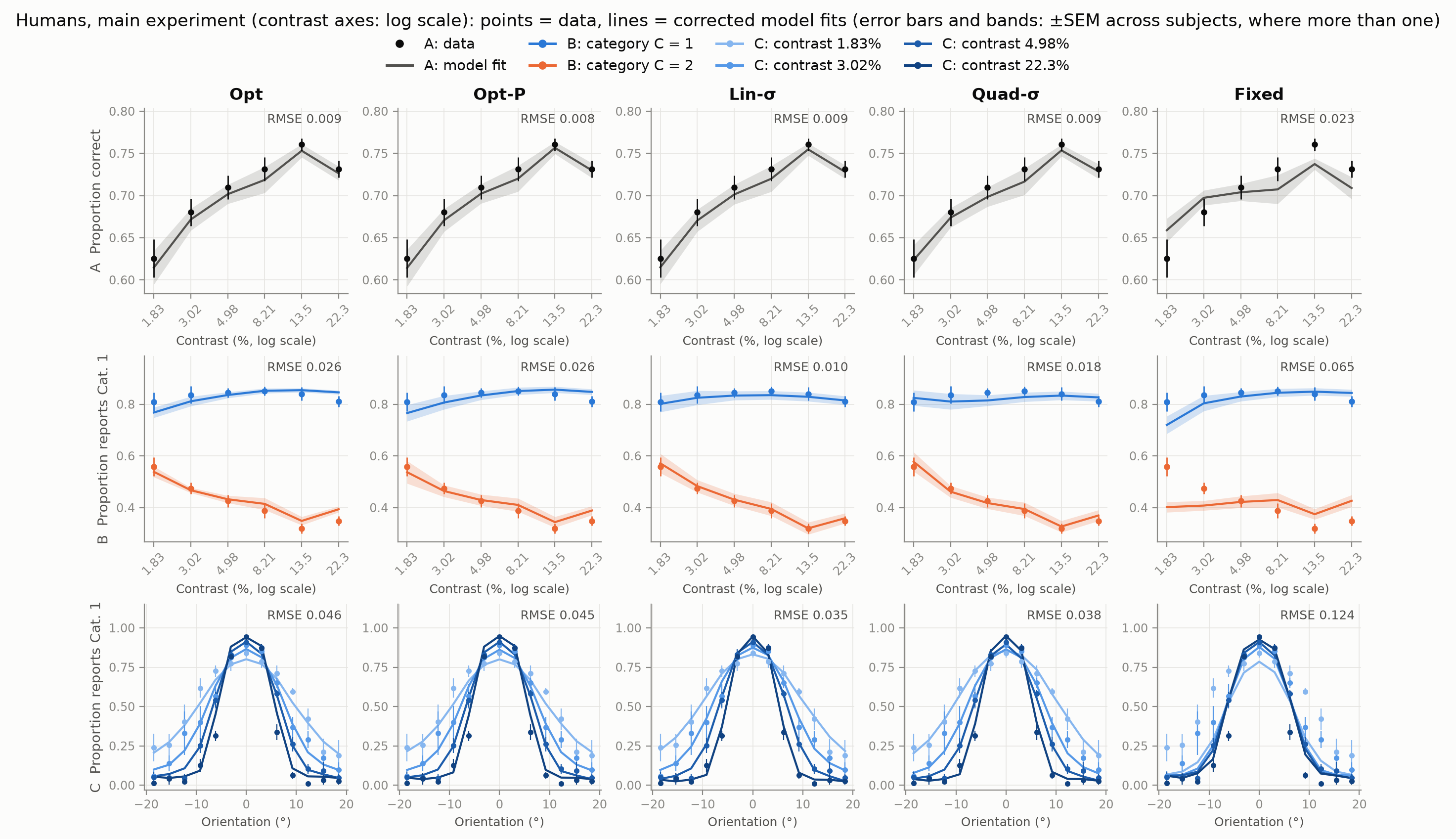
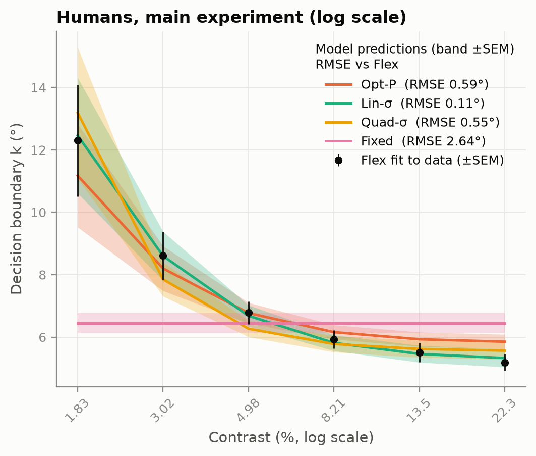
Figures and statistics: the Fig 2A/2C and 3A/3C psychometric RMSEs are identical at the archived parameters. The Fig 2D boundary RMSEs are Opt-P , Lin-σ , Quad-σ , Fixed (published 0.59 / 0.11 / 0.55 / 2.64). The repeated-measures ANOVA gives F(5,25) = (published 12.4). The Fig 2E correlation is r = (published 0.89).
One exception, explained: the published Fig 2B/3B RMSEs are exactly √2 × what the archived plotting code produces. The archived code's own saved figures show our values, so the published panel came from a different code version (audit D8).

Code audit

Each item was checked numerically and confirmed by an independent reviewer agent before it was reported. "Severity" is how much the item matters for the published results: High changes a published number materially or the wording of a claim; Medium numbers move but conclusions hold; Low negligible; Doc documentation. Our own bug is listed too.

#	Severity	Finding	Status	Impact

Corrected vs published model comparison

The corrected analysis fixes the gradient bug, uses 1,000 starts per fit (the protocol the SI describes), keeps parameters inside the SI's prior box, uses exact Hessians, and adds nested-sampling evidence, which stays valid where the Laplace approximation breaks (optima on a parameter bound or a non-positive-definite Hessian). The chart shows each model's evidence relative to the best model for that subject. The shaded band is the paper's "within $\log 30$ " criterion for the set of best models.

Log evidence relative to the best model

Triangles mark values beyond the axis (Fixed for the monkeys is 1,700–2,600 below the best). Hover a row for all five values.

Table view (corrected, with change vs published)

Decision boundaries by contrast

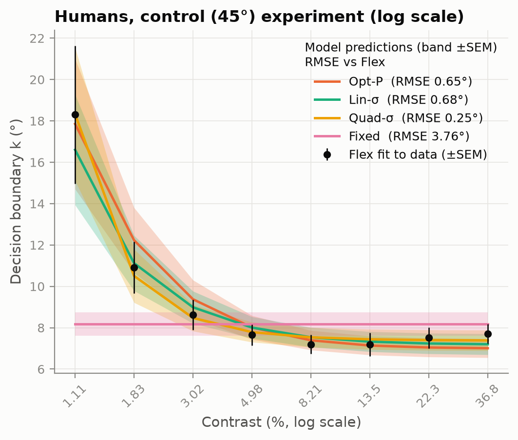
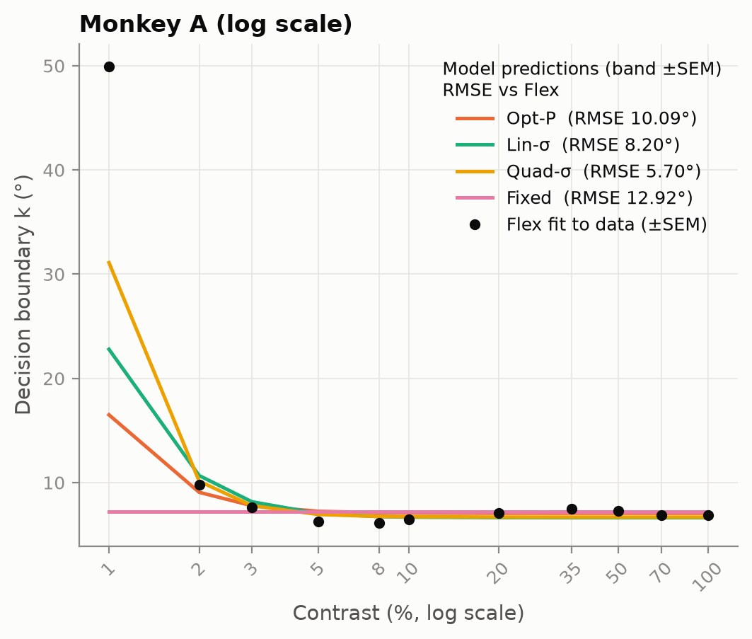
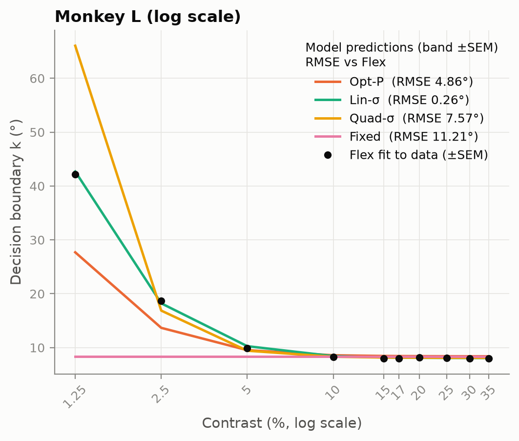
The "Flex" model fits a free boundary at every contrast, a model-free estimate of where each observer put the boundary. The parametric models' boundaries can then be compared with it (Fig 2D in the paper). Choose a dataset and a subject.

Boundary k vs contrast (log x)

Dots: Flex estimates. Lines: boundaries predicted by each fitted model (corrected fits). RMSE vs Flex across subjects, in degrees:

What changed in the conclusions

Headline: nothing major changed. Every main conclusion survives the corrections. Fixed is never the best model. Subjects remain split across Opt, Opt-P, Lin-σ and Quad-σ. Monkey A prefers Quad-σ and Monkey L prefers Lin-σ. No winner is changed by a correction.

Correction	Effect on numbers	Effect on conclusions
$\sigma_p$ gradient bug fixed, better optimiser (B1, B2)	Monkey A Lin-σ log-likelihood +111.6; Monkey L Lin-σ +16.5, Quad-σ +2.2; humans ≤ 0.5	Winners unchanged. Monkey A's Quad-σ margin over Lin-σ shrinks from 192 to 82 nats; Monkey L's Lin-σ margin over Quad-σ grows from 38 to 52.
Laplace invalid on ridge/boundary optima (B3), replaced by nested sampling	Monkey A Lin-σ evidence −32,954 → −32,844	None (Quad-σ still best by 82 nats)
SI prior box enforced (D2, D7)	Fixed log evidence −1.2 ( $k_0$ range 50 instead of 15); a few fits move by ≤ 0.04	None
RG's discrimination session: the analysis used a pilot session (B6)	Fig 2E r: → ( pooled)	Slightly stronger
Within-contrast σ agreement (D9, M1)	Per-contrast across-subject r (n = 6) has 95% CIs spanning about −0.6 to 0.9; contrast-demeaned r =	Subject-level validation is inconclusive at n = 6; the pooled r mostly reflects the shared contrast trend
Sphericity correction for the boundary ANOVA (M3)	Greenhouse–Geisser $\varepsilon$ = ; p: 4×10⁻⁶ →	Effect survives, evidence much weaker than "P < 10⁻⁵"
Opt-P: $k = 0$ instead of "infeasible" (B4)	No optimum moved ( $\|\Delta \mathrm{LL}\| \le 10^{-4}$ )	None

Qualifications

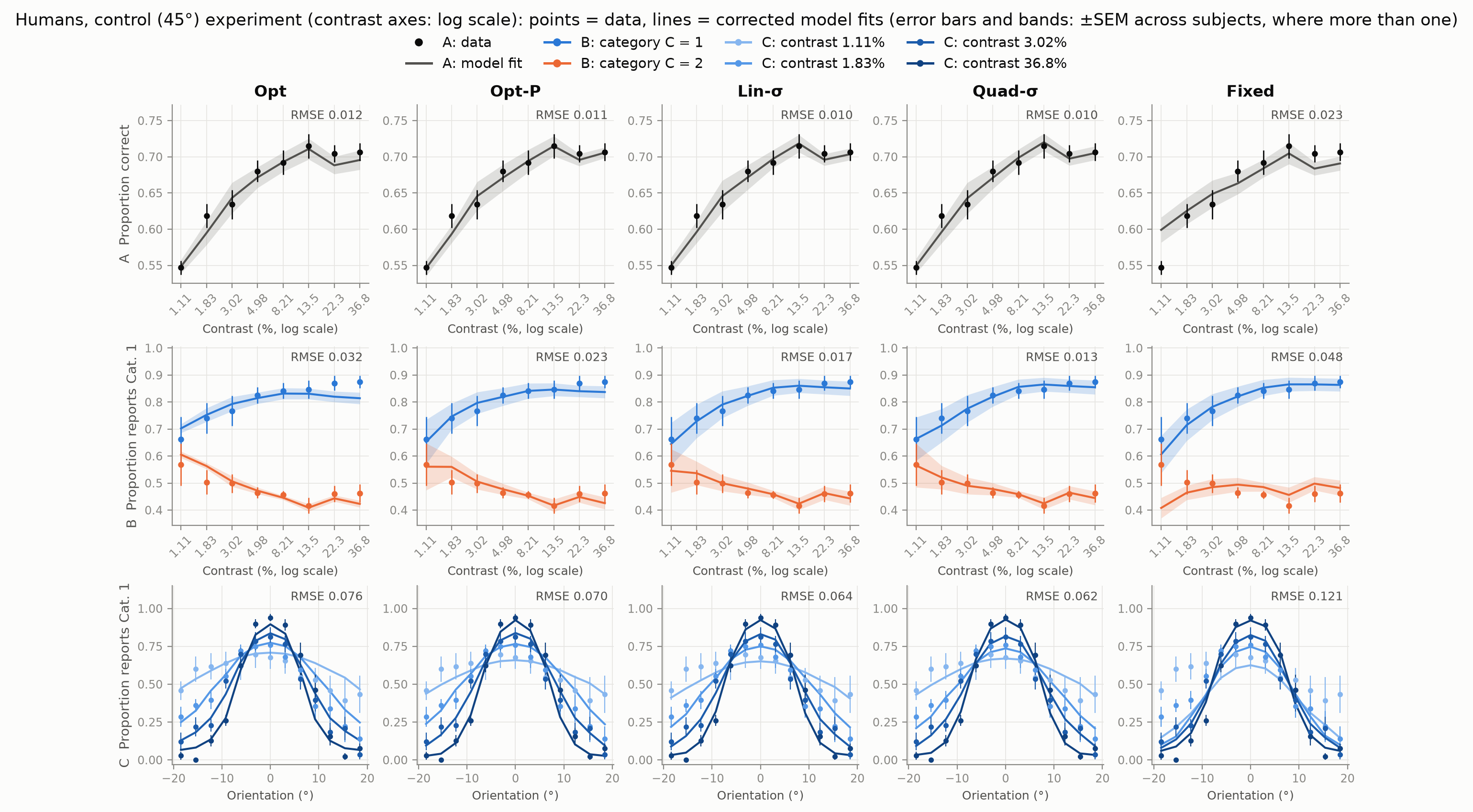
Control experiment: Fixed is within $\log 30$ of the best model for subject NL. This is also true in the published Table S4 (DIFF −1.9), contrary to the text's "Fixed is never among them".
Independent σ: the discrimination-task σ agrees with the categorisation σ across contrasts, but across the six subjects the agreement is inconclusive, not demonstrated.
ANOVA: the boundary-vs-contrast effect survives the sphericity correction only at p = 0.016.

Control subject JO shows Lin-σ in the published Table S4 but Quad-σ in both the archived 2013 fit file and our corrected fit. The difference comes from the published control tables disagreeing with the archived fits (D3), not from our corrections; the two models are 1.3 nats apart.

Figures

Regenerated from the corrected fits. Psychometric curves: proportion of "category 1" reports vs orientation, by contrast (data points, model curves).

Psychometric curves, humans main experiment — Humans, main experiment (Fig 2A–C equivalent).

Boundary vs contrast, humans main experiment — Boundaries, humans, main experiment (Fig 2D equivalent).

Psychometric curves, humans control experiment — Humans, control experiment (45° rotated categories).

Psychometric curves, Monkey A — Monkey A (Fig 3 equivalent).

Psychometric curves, Monkey L — Monkey L.